
Let’s pretend you have a spreadsheet with 1,000 rows of data — it would be pretty difficult to spot patterns in the data with the naked eye. Enter conditional formatting.
This powerful tool highlights cells that meet a specific condition or “rule.” In other words, it brings your spreadsheet to life by adding color to patterns and trends.

Here, we’ll cover how to apply, edit, and copy and paste conditional formatting.
Conditional Formatting Based on Text
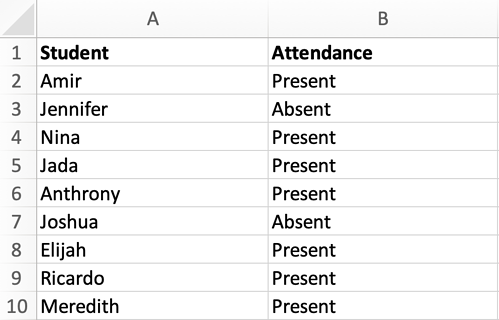
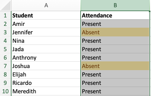
In this example, let’s use conditional formatting to an attendance list to highlight who was absent. The image below is the data set I’ll use to run through this explanation:
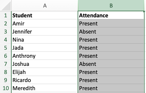
1. First, select the column or row you want to apply conditional formatting to. In this case, we’ll select column B.
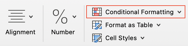
2. To highlight who was absent, navigate to the header toolbar and select Conditional Formatting, as shown in the image below.
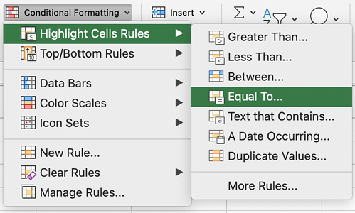
3. When the Conditional Formatting drop-down menu appears, select Highlight Cells Rules, then Equal To.
4. In the New Formatting dialog box, change Cell Value to Specific Text. Then, type “Absent” in the text box. Reference the image below:
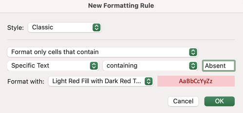
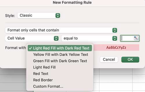
5. From the New Formatting dialog box, we can also choose how we want to format the cells containing the word “Absent.” Check out the options below.
For this example, let’s stick with the default option (Light Red Fill with Dark Red Text).
6. Click OK. Now — thanks to conditional formatting — we can quickly identify which students were absent.
In the next section, we’ll cover how to apply conditional formatting based on another cell in the spreadsheet.
Conditional Formatting Based on Another Cell
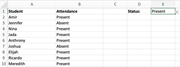
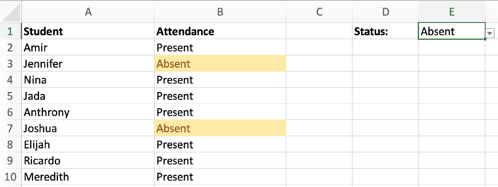
In this example, the goal is to highlight the cells that match the drop-down menu in cell E1. The image below is the sample data set I’ll use for this explanation:
1. First, select column B.
2. Navigate to the header toolbar and select Conditional Formatting. When the Conditional Formatting drop-down menu appears, select Highlight Cells Rules, then Equal To.
3. In the New Formatting dialog box, select Cell Value and Equal To.
In the text box, you can either click your mouse on cell E1 (the cell that contains the drop-down menu), or manually enter the formula =$E$1. See below.
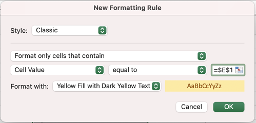
4. As you can see in the image above, we also changed the formatting to Yellow Fill with Dark Yellow Text. However, you can change this option to your preference. Click OK.
5. Now, the cells that match cell E1 are highlighted in yellow. Notice how the highlighted cells change depending on the status:
- When the status is Present:
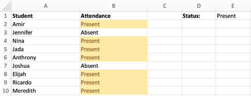
- When the status is Absent:
How to Edit Conditional Formatting
Here’s some good news — conditional formatting is not set in stone, meaning you can edit or delete it later. Here are the steps to do that:
1. Start by selecting the cell (or cell range) that contains a conditional formatting rule.
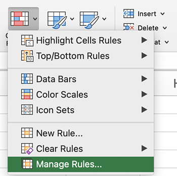
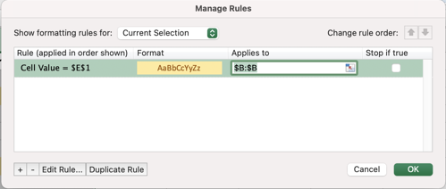
2. Navigate to the header toolbar and select Conditional Formatting, then Manage Rules.
3. The Manage Rules dialog box will list the current rules for your selection. Select the rule you want to edit and click Edit Rule.
How to Copy Conditional Formatting in Excel
You can easily copy a conditional formatting rule to another cell to (or range of cells) by using one of the following approaches.
1. Simple copy/paste.
The first approach is relatively straightforward. Start by selecting the cell you want to copy and hit the Copy button in the header toolbar — or click Control-C (or Command-C on a Mac).
Then, select the target cell and hit the Paste button in the header toolbar, or click Control-V (or Command-V on a Mac).
2. Format Painter
The second approach uses the tool Format Painter, which is located in the header toolbar. Check out the image below:

To start, click on the cell you want to copy, then click Format Painter. Your mouse icon will change to a paintbrush. Then, drag the paintbrush to the cell (or range of cells) where you want to paste the format. Lastly, to stop using the paintbrush, press Esc on your keyboard.
Conditional formatting is a powerful way to visualize the data in your spreadsheet. With just a few clicks, you can emphasize important trends or patterns you may have otherwise missed. With the tips in this post, you’ll be able to use Conditional Formatting to its fullest extent.