
Microsoft Excel is a very powerful multi-purpose tool that anyone can use. But if you’re someone who works with spreadsheets every day, you might need to know more than just the basics of using Excel. Knowing a few simple tricks can go a long way with Excel. A good example is knowing how to link cells in Excel between sheets and workbooks.
Learning this will save a lot of time and confusion in the long run.

Why Link Cell Data in Excel
Being able to reference data across different sheets is a valuable skill for a few reasons.
First, it will make it easier to organize your spreadsheets. For example, you can use one sheet or workbook for collecting raw data, and then create a new tab or a new workbook for reports and/or summations.
Once you link the cells between the two, you only need to change or enter new data in one of them and the results will automatically change in the other. All without having to move back and forth between different spreadsheets.

Second, this trick will avoid duplicating the same numbers in multiple spreadsheets. This will reduce your working time and the possibility of making calculation mistakes.
In the following article, you’ll learn how to link single cells in other worksheets, link a range of cells, and how to link cells from different Excel documents.
How to Link Two Single Cells
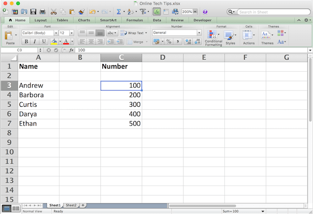
Let’s start by linking two cells located in different sheets (or tabs) but in the same Excel file. In order to do that, follow these steps.

- In Sheet2 type an equal symbol (=) into a cell.
- Go to the other tab (Sheet1) and click the cell that you want to link to.
- Press Enter to complete the formula.
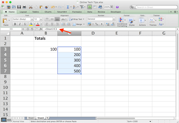
Now, if you click on the cell in Sheet2, you’ll see that Excel writes the path for you in the formula bar.
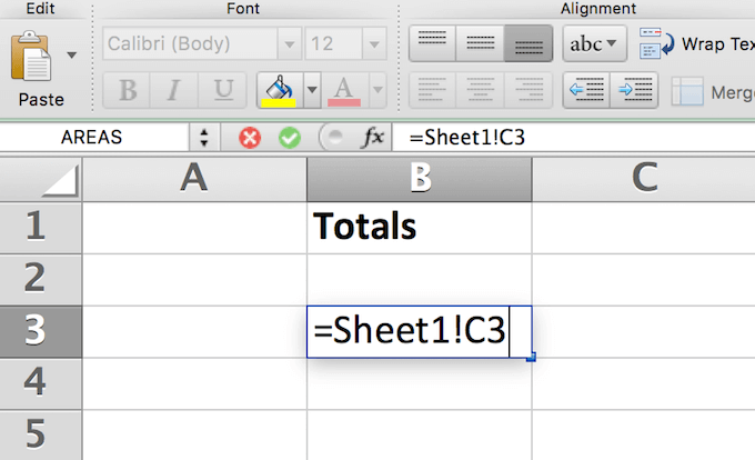
For example, =Sheet1!C3, where Sheet1 is the name of the sheet, C3 is the cell you’re linking to, and the exclamation mark (!) is used as a separator between the two.
Using this approach, you can link manually without leaving the original worksheet at all. Just type the reference formula directly into the cell.
Note: If the sheet name contains spaces (for example Sheet 1), then you need to put the name in single quotation marks when typing the reference into a cell. Like =’Sheet 1′!C3. That’s why it’s sometimes easier and more reliable to let Excel write the reference formula for you.
How to Link a Range of Cells
Another way you can link cells in Excel is by linking a whole range of cells from different Excel tabs. This is useful when you need to store the same data in different sheets without having to edit both sheets.
In order to link more than one cell in Excel, follow these steps.
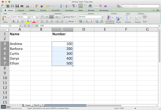
- In the original tab with data (Sheet1), highlight the cells that you want to reference.
- Copy the cells (Ctrl/Command + C, or right click and choose Copy).
- Go to the other tab (Sheet2) and click on the cell (or cells) where you want to place the links.

- Right click on the cell(-s) and select Paste Special…
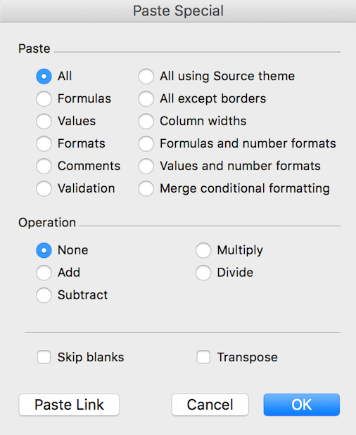
- At the bottom left corner of the menu choose Paste Link.
When you click on the newly linked cells in Sheet2 you can see the references to the cells from Sheet1 in the formula tab. Now, whenever you change the data in the chosen cells in Sheet1, it will automatically change the data in the linked cells in Sheet2.
How to Link a Cell With a Function
Linking to a cluster of cells can be useful when you do summations and want to keep them on a sheet separate from the original raw data.
Let’s say you need to write a SUM function in Sheet2 that will link to a number of cells from Sheet1. In order to do that, go to Sheet2 and click on the cell where you want to place the function. Write the function as normal, but when it comes to choosing the range of cells, go to the other sheet and highlight them as described above.
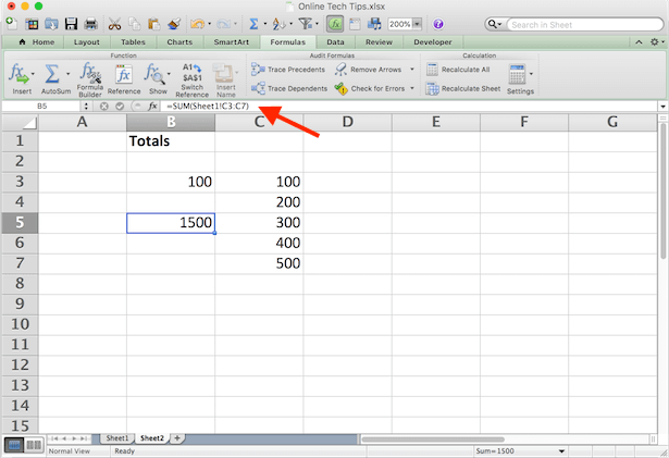
You will have =SUM(Sheet1!C3:C7), where the SUM function sums the contents from cells C3:C7 in Sheet1. Press Enter to complete the formula.
How to Link Cells From Different Excel Files
The process of linking between different Excel files (or workbooks) is virtually the same as above. Except, when you paste the cells, paste them in a different spreadsheet instead of a different tab. Here’s how to do it in 4 easy steps.
- Open both Excel documents.
- In the second file (Help Desk Geek), choose a cell and type an equal symbol (=).
- Switch to the original file (Online Tech Tips), and click on the cell that you want to link to.
- Press Enter to complete the formula.
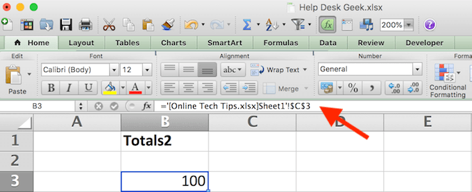
Now the formula for the linked cell also has the other workbook name in square brackets.

If you close the original Excel file and look at the formula again, you will see that it now also has the entire document’s location. Meaning that if you move the original file that you linked to another place or rename it, the links will stop working. That’s why it’s more reliable to keep all the important data in the same Excel file.
Become a Pro Microsoft Excel User
Linking cells between sheets is only one example of how you can filter data in Excel and keep your spreadsheets organized. Check out some other Excel tips and tricks that we put together to help you become an advanced user.
What other neat Excel lifehacks do you know and use? Do you know any other creative ways to link cells in Excel? Share them with us in the comment section below.