

If you’ve never spent time using Microsoft Excel, it can feel a bit overwhelming at first. We’ll teach you the basic tasks you need to know to use this popular spreadsheet application.
From entering data and formatting numbers to adding cell borders and shading, knowing these essentials will ease the stress of learning to use Excel.
Entering Data in Excel
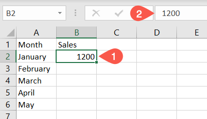
You have two easy ways to enter data in the cells of an Excel sheet.
First, you can click the cell and type your data into it. Second, you can click the cell and type the data into the Formula Bar which is at the top of the sheet.
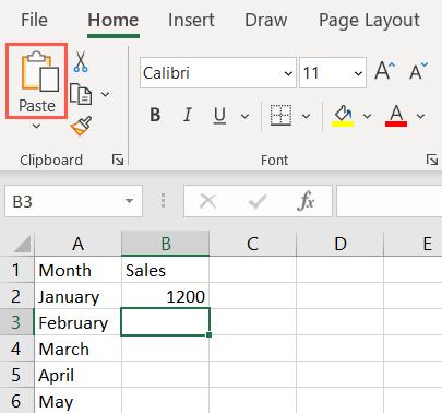
You can also copy data from another location and paste it in your sheet. Once you copy it, select the cell in your sheet and paste it by doing one of the following:
- Use the keyboard shortcut Ctrl+V on Windows or Command+V on Mac.
- Click “Paste” in the Clipboard section on the Home tab.
- Right-click the cell and pick “Paste” in the shortcut menu.
For more ways to paste like multiplying numbers as you do, look at our how-to on using Paste Special in Excel.
Managing Spreadsheets
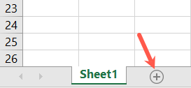
You can add many sheets to your Excel workbook. This is handy for handling projects that require separate spreadsheets.
To add a sheet, click the plus sign on the far-right side of the sheet tab row. This adds a spreadsheet to the right of the active one.
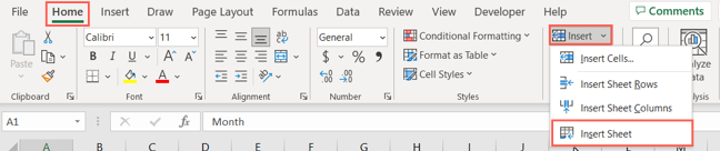
Alternatively, go to the Home tab, select the Insert drop-down box in the Cells section of the ribbon, and pick “Insert Sheet.” This adds a spreadsheet to the left of the active one.
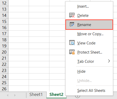
When you add a sheet, it has a default name of Sheet with a number. So, you’ll see Sheet1, Sheet2, and so on. To rename a sheet, double-click the current name or right-click and pick “Rename.” Then, type the new name and press Enter or Return.
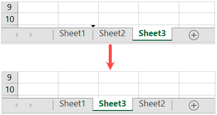
To rearrange sheets, select one and drag it left or right to the spot where you want it. Then, release.
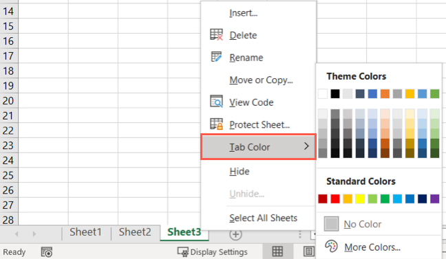
To color the tab for a sheet, right-click the tab, move to Tab Color, and select a color in the pop-out menu. This is a great way to spot certain sheets at a glance or color-code them for specific tasks.
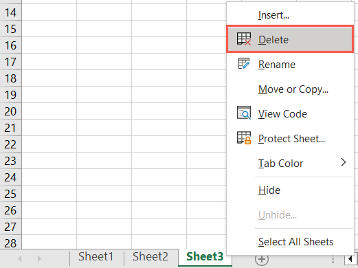
To remove a sheet, right-click and choose “Delete.” If the sheet contains data, you’ll be asked to confirm that you want to delete the sheet and the data. Select “Delete” to continue or “Cancel” to keep the sheet.
Adding and Removing Columns and Rows
You may discover that you need an additional column or row within your data set. Or, you might decide to remove a column or row you no longer need.
Add a Column or Row
You can insert a column or row a couple of different ways.
- Right-click a column or row and choose “Insert” from the shortcut menu.
- Select a column or row and go to the Home tab. Open the Insert drop-down box in the Cells section and pick “Insert Sheet Rows” or “Insert Sheet Columns.”
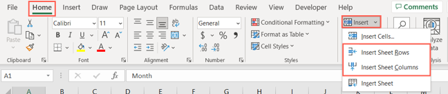
Both of the above actions insert a column to the left of the selected column or a row above the selected row.
Remove a Column or Row
To remove a column or row, you can use similar actions. To select a column, click the column header which is the letter at the top. To select a row, click the row header which is the number on the left.
- Right-click the column or row and choose “Delete” from the shortcut menu.
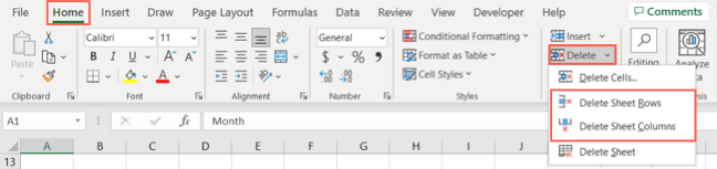
- Select the column or row and go to the Home tab. Open the Delete drop-down box in the Cells section and pick “Delete Sheet Rows” or “Delete Sheet Columns.”
For more, look at our tutorial for inserting multiple rows in Excel.
Formatting Numbers
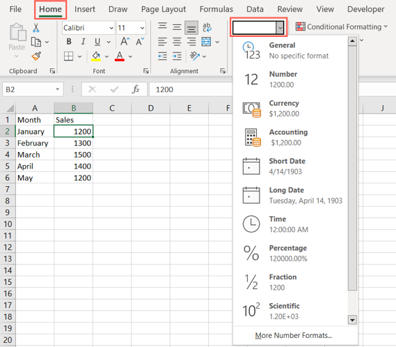
When you enter numbers in Excel, you can format them as ordinary numbers, currencies, decimals, percentages, dates, times, and fractions.
Select a cell, go to the Home tab, and use the drop-down box in the Number section of the ribbon to pick the format. As you review the list of options, you’ll see examples of how the data will appear.
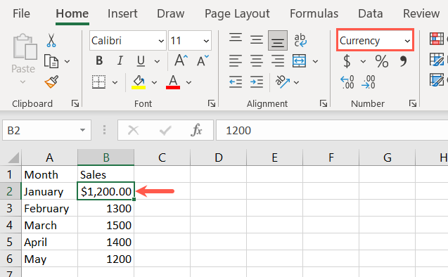
Pick the format you want, and you’ll see your data update.
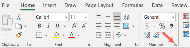
You can also choose the style for the number format you use. Click the small arrow on the bottom right of the Number section in the ribbon.
When the Format Cells box appears, go to the Number tab and select an option on the left.
On the right, you’ll see a preview of the format with options below you can adjust. For example, you can choose the number of decimal places and how you want to display negative numbers.
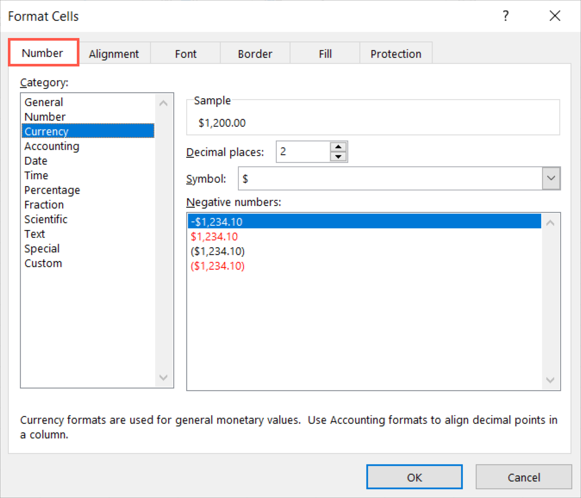
After you make your selections, click “OK” to apply them to the value.
Formatting Fonts and Cells
Along with formatting the data within a cell, you can format the cell itself. You may want to use a specific font style, apply a cell border, or add shading to a cell.
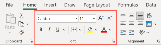
Select the cell you want to change and head to the Home tab. You’ll see several options in the Font section of the ribbon.
Font style and size: Use the drop-down boxes at the top to change the font style or size. You can also use the buttons to the right to increase or decrease the font size.
Bold, italics, and underline: Simply select one of these buttons to apply bold, italics, or underline to the font in a cell.
Border: Use the Border drop-down box to choose the type and style for the cell border.
Fill and font colors: Select the Fill Color drop-down box to pick a color for the cell or the Font Color box to pick a color for the font.
Performing Quick Calculations
When you work with numbers in your sheet, it’s common to perform calculations. Rather than delve into creating formulas in Excel, which is a bit more advanced, you can quickly add, average, or get the minimum or maximum number in a data set.
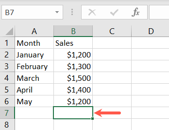
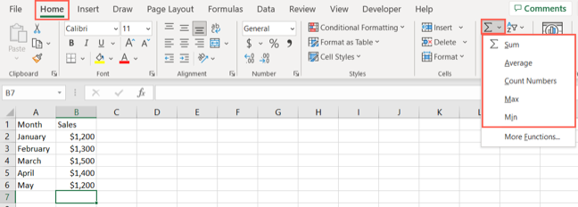
Go to the cell where you want to add the calculation. As an example, we’ll sum the cells B2 through B6, so we pick cell B7.
Head to the Home tab and select the Sum drop-down box in the Editing section of the ribbon. You’ll see the basic calculations you can perform. For our example, we select “Sum.”
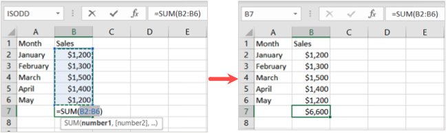
You’ll then see Excel highlight the cells it believes you want to calculate. It also shows you the function and formula it’ll use. Simply press Enter or Return to accept the suggestion and get the result.
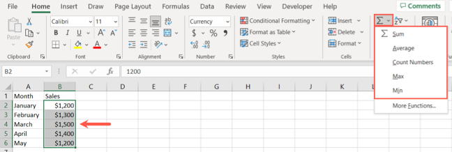
Alternatively, you can start by selecting the cells you want to calculate. Then, choose the calculation from the Sum drop-down box.
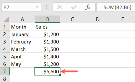
You’ll see the result of the calculation below cells in a column or to the right of cells in a row.
As an Excel beginner, these basic tasks should get you off to a great start using the application. Once you master these actions, be sure to check out our additional Excel articles for things like creating a graph, using a table, and sorting or filtering data.