
If you are a finance professional or a finance student, you might have heard about the Gantt Chart. It is a horizontal bar chart that is most commonly used in project management and planning. It shows the entire project on a timeline. This is its most significant benefit. The Gantt Chart helps you analyze the following data:
- Beginning and end of each task,
- The total duration of each task,
- Deadlines of the project,
- The complete schedule of the projects from beginning to end, and more.
In this article, we will discuss the steps to create a Gantt Chart in Google Sheets.
How to make a Gantt Chart in Google Sheets
1] First, you have to create a new project in Google Sheets. Type your project data in three columns. Here, we have classified the data as Project Name, Start Date, and End Date. You can enter the data as per your choice. Now, complete your table by entering the project names and start and end dates.

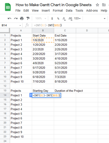
2] Now, copy the first column and paste it below the table you created, leaving one row in between. Name the second column of the new table as Starting Day and the third column as Duration of the Project. See the below screenshot.

3] You have to apply a formula in the second column of the second table. For this, select the cell next to Project 1 in the second table. In our case, it is cell number B14. Write the following formula there and press Enter:
=INT(B2)-INT($B$2)
Do note that, in the above formula, we wrote B2 because the start date of Project 1 lies in the B2 cell. You can set change the cell number in the formula as per your table.
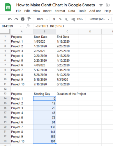
4] Place your cursor on the bottom right corner of the selected cell (in this case, it is B14). When your cursor changes to the Plus icon, drag it to the last cell. This will copy and paste the entire formula to all the cells and give you the final values.
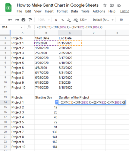
5] Select the cell just below the Duration of the Project cell. Enter the following formula and press Enter:
=(INT(C2)-INT($B$2))-(INT(B2)-INT($B$2)
Please fill the cell address in the formula correctly (as described in step 3); otherwise, you will get an error.
6] Now, place your cursor on the bottom right corner of the same cell and drag it to the end. This will copy and paste the entire formula to all the cells, and you will get the final values.

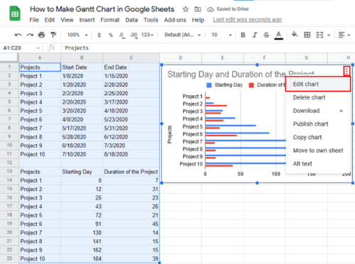
7] Now, you have to insert a Stacked Bar Chart. For this, select both the tables and go to “Insert > Chart.” You will get a normal bar graph.

8] You have to change the normal bar graph to Stacked Bar Chart. Select the chart, click on the three vertical dots on the top right side, and then click on the “Edit Chart” option. This will open the chart editing window on the right side of the Google Sheets.
9] Click on the “Set Up” tab. After that, click on the drop-down menu in the “Chart Type.” Now, scroll down and select the middle chart in the “Bar” section. This will change the normal bar graph to the Stacked Bar Chart.

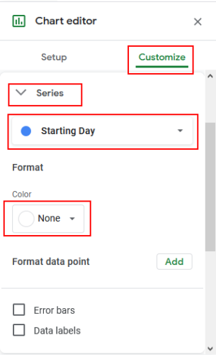
10] Now, go to the “Customize” tab and expand the “Series” section. Select “Starting Day” in the drop-down menu. After that, click on the “Color” drop-down menu and select “None.”
Your Gantt Chart is ready. If you want, you can make it 3D using the “Customize” option.

We hope this article helped you create a Gantt Chart.
You may also like: How to create Gantt Chart using Microsoft Excel.
