
When you need to find a value’s exact position in your spreadsheet, you can use the MATCH function in Excel. This saves you from manually searching for the location that you may need for reference or another formula.
The MATCH function is often used with the INDEX function as an advanced lookup. But here, we’ll walk through how to use MATCH on its own to find a value’s spot.
What Is the MATCH Function in Excel?
The MATCH function in Excel searches for a value in the array, or range of cells, that you specify.
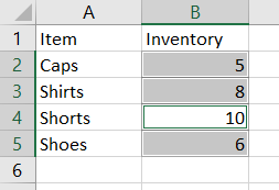
For instance, you might look up the value 10 in the cell range B2 through B5. Using MATCH in a formula, the result would be 3 because the value 10 is in the third position of that array.
The syntax for the function is MATCH(value, array, match_type) where the first two arguments are required and match_type is optional.
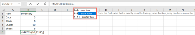
The match type can be one of the following three options. If the argument is omitted from the formula, 1 is used by default.
- 1: Finds the largest value less than or equal to the searched
value. The range must be in ascending order. - 0: Finds the value exactly equal to the searched
valueand the range can be in any order. - -1: Finds the smallest value greater than or equal to the searched
value. The range must be in descending order.
You may also see these match types as a tooltip when you build your formula in Excel.
The MATCH function is not case sensitive, allows the wildcards asterisk (*) and question mark (?), and returns #N/A as the error if no match is found.
Use MATCH in Excel
When you’re ready to put the MATCH function to work, take a look at these examples to help you walk through building the formula.
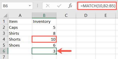
Using our example above, you would use this formula to find the value 10 in the range B2 through B5. Again, our result is 3 representing the third position in the cell range.
=MATCH(10,B2:B5)
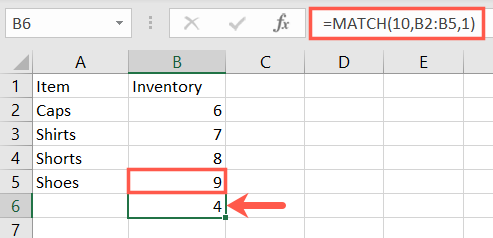
For another example, we’ll include the match type 1 at the end of our formula. Remember, match type 1 requires the array be in ascending order.
=MATCH(10,B2:B5,1)
The result is 4 which is the position of the number 9 in our range. That’s the highest value less than or equal to 10.
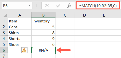
Here’s an example using match type 0 for an exact match. As you can see, we receive the #N/A error because there is no exact match to our value.
=MATCH(10,B2:B5,0)
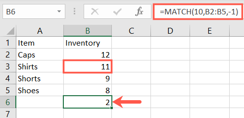
Let’s use the final match type -1 in this formula.
=MATCH(10,B2:B5,-1)
The result is 2 which is the position of the number 11 in our range. That’s the lowest value greater than or equal to 10. Again, match type -1 requires the array be in descending order.
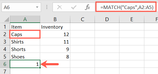
For an example using text, here we can find Caps in the cell range A2 through A5. The result is 1 which is the first position in our array.
=MATCH("Caps",A2:A5)
Now that you know the basics of using the MATCH function in Excel, you might also be interested in learning about using XLOOKUP in Excel or using VLOOKUP for a range of values.