
Dupliserte data er forbannelsen av regnearkløsninger, spesielt i stor skala. Gitt volumet og variasjonen av data som nå legges inn av team, er det mulig at duplisere data i verktøy somGoogle Sheetskan være relevant og nødvendig, eller det kan være en frustrerende distraksjon fra hovedformålet med regnearkarbeid.
Det potensielle problemet reiser et godt spørsmål: Hvordan fremhever du duplikater i Google Sheets?
Vi har dekket deg med en trinnvis titt på hvordan du fremhever duplikater i Google Sheets, komplett med bilder for å sikre at du er på rett spor når det gjelder å deduplisere dataene dine.
Fremhev dupliserte data i Google Sheets
Google Sheets er et gratis, skybasert alternativ til proprietære regnearkprogrammer og – ingen overraskelse, siden det er Google vi har å gjøre med – tilbyr en rekke flotte funksjoner for å effektivisere datainntasting, formatering og beregninger.

Google Sheets har alle de kjente funksjonene: Fil, Rediger, Vis, Formater, Data, Verktøy osv. og gjør det enkelt å raskt legge inn data, legge tilformlerfor beregninger, og oppdage sentrale sammenhenger. Det Sheets imidlertid ikke har, er en enkel måte å finne og fremheve duplikater.
Mens andre regnearkverktøy,som Excel, har innebygde betingede formateringsverktøy som kan finne dupliserte data i arket ditt, krever Googles løsning litt mer manuell innsats.
Trinn-for-trinn: Slik markerer du duplikater i Google Sheets (med bilder)
Så hvordan fremhever du automatisk duplikater i Google Sheets? Selv om det ikke er noe innebygd verktøy for dette formålet, kan du bruke noen innebygde funksjoner for å fremheve dupliserte data.
Her er en steg-for-steg guide:
Trinn 1: Åpne regnearket.
Trinn 2: Marker dataene du vil sjekke.
Trinn 3: Under "Format", velg "Betinget formatering."
Trinn 4: Velg "Egendefinert formel er."
Trinn 5: Skriv inn den tilpassede duplikatkontrollformelen.
Trinn 6: Klikk "Ferdig" for å se resultatene.
Trinn 1: Åpne regnearket.
Gå først til Google Sheets og åpne regnearket du vil se etter dupliserte data.
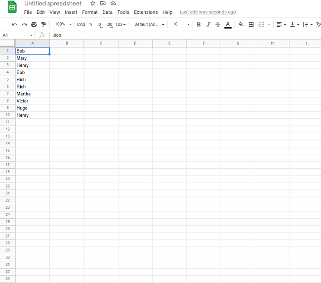
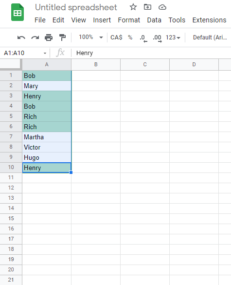
Trinn 2: Marker dataene du vil sjekke.
Deretter venstreklikker du og drar markøren over dataene du vil sjekke for å markere dem.

Trinn 3: Under "Format", velg "Betinget formatering."
Gå nå til "Format" i den øverste menyraden og velg "Betinget formatering". Du kan få et varsel som sier "cellen er ikke tom" - hvis ja, klikk på den, og du bør se dette:

Trinn 4: Velg "Egendefinert formel er."
Deretter må vi lage en tilpasset formel. Under "Formater celler hvis", velg rullegardinmenyen og rull ned til "Egendefinert formel er".

Trinn 5: Skriv inn den tilpassede duplikatkontrollformelen.
For å søke etter dupliserte data, må vi angi den tilpassede duplikatkontrollformelen, som for vår datakolonne ser slik ut:
=ANTALLHVIS(A:A,A1)>1
Denne formelen søker etter en hvilken som helst tekststreng som vises mer enn én gang i vårt valgte datasett, og vil som standard utheve den i grønt. Hvis du foretrekker en annen farge, klikker du på det lille malekarikonet i formateringsstillinjen og velger fargen du foretrekker.

Trinn 6: Klikk "Ferdig" for å se resultatene.
Og voilà – vi har fremhevet dupliserte data i Google Sheets.
Slik markerer du duplikater i flere rader og kolonner
Hvis du har et større datasett å sjekke, er det også mulig å markere dataduplikater i flere kolonner eller rader.
Dette starter på samme måte som duplikatkontrollprosessen ovenfor - den eneste forskjellen er at du endrer dataområdet til å inkludere alle cellene du vil sammenligne.
I praksis betyr dette å legge inn et utvidet dataområde i menyen Betingede formatregler og boksen for tilpasset format. La oss bruke eksempelet ovenfor som et utgangspunkt, men i stedet for bare å søke i kolonne A etter duplikater, skal vi søke på tvers av tre kolonner: A, B og C, og også på tvers av radene 1-10.
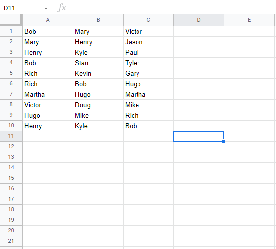
Når vi legger inn reglene for betinget format, blir Apply to Range A1:C10 og vår egendefinerte formel blir:
=COUNTIF($A$2:G,Indirect(Address(Row(),Column(),)))>1
Dette vil fremheve alle duplikater på tvers av alle tre kolonnene og alle 10 radene, noe som gjør det enkelt å oppdage datadoppelgangere:

Håndtere duplikater i duplikater i Google Sheets
Kan du markere duplikater i Google Sheets? Absolutt. Selv om prosessen krever mer innsats enn noen andre regnearkløsninger, er den lett å replikere når du har gjort den en eller to ganger, og når du er komfortabel med prosessen kan du skalere opp for å finne duplikater på tvers av rader, kolonner og til og med mye større datasett.