

To multiply columns in Excel, use a formula that includes two cell references separated by the multiplication operator (asterisk). Then, use the fill handle to copy the formula to all other cells in the column. You can also use the PRODUCT function, an array formula, or the Paste Special feature.
Microsoft Excel is full of useful features, including those for performing calculations. If there comes a time when you need to multiply two columns in Excel, there are various methods for doing so. We’ll show you how to multiply columns right here.
How to Multiply a Column in Excel
To multiply columns in Excel, you can use an operator, function, formula, or feature to tackle the task. Let’s jump in.
Use the Multiplication Operator
Just like multiplying a single set of numbers with the multiplication operator (asterisk), you can do the same for values in columns using the cell references. Then, use the fill handle to copy the formula to the rest of the column.
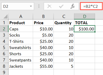
Select the cell at the top of the output range, which is the area where you want the results. Then, enter the multiplication formula using the cell references and asterisk. For example, we’ll multiply two columns starting with cells B2 and C2 and this formula:
=B2*C2
When you press Enter, you’ll see the result from your multiplication formula.
You can then copy the formula to the remaining cells in the column. Select the cell containing the formula and double-click the fill handle (green square) in the bottom right corner.
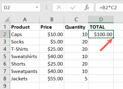
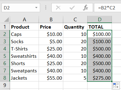
The empty cells below fill with the formula and the cell references adjust automatically. You can also drag the handle down to fill the remaining cells instead of double-clicking it.
Note: If you use absolute cell references instead of relative ones, they will not automatically update when you copy and paste the formula.
Pull in the PRODUCT Function
Another good way to multiply columns in Excel is using the PRODUCT function. This function works just like the multiplication operator. It’s most beneficial when you need to multiply many values, but it works just fine in Excel to multiply columns.
The syntax for the function is PRODUCT(value1, value2,...) where you can use cell references or numbers for the arguments. For multiplying columns, you’ll use the former.
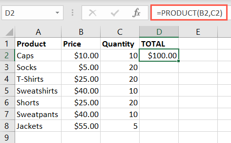
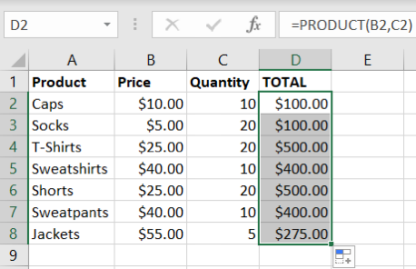
Using the same example above, you start by entering the formula and then copy it down to the remaining cells. So, to multiply the values in cells B2 and C2, you’d use this formula:
=PRODUCT(B2,C2)
Once you receive your result, double-click the fill handle or drag it down to fill the rest of the column with your formula. Again, you’ll see the relative cell references adjust automatically.
Create an Array Formula
If you want to remove the “fill formula” step from the process, consider using an array formula to multiply your columns. With this type of formula, you can perform your calculation for all values in one fell swoop.
There’s a slight difference in how you apply array formulas in Excel 365 compared to other versions of Excel.
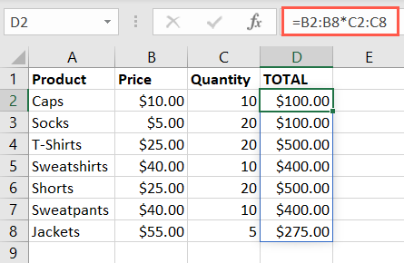
For Excel 365, enter the array formula in the top-left cell of your output range. The formula begins with an equal sign (=) and includes the first cell range, an asterisk for multiplication, and the second cell range. Once you enter the formula, press Enter to apply it.
Using our example, we’ll multiply the cell range B2 through B8 by C2 through C8 using this formula:
=B2:B8*C2:C8
As you’ll see, this fills your column with the multiplication results all at once.
For other Excel versions, you use the same formula but apply it a bit differently. Select the output range, enter the array formula in the top-left cell of that range, and then press Ctrl+Shift+Enter.
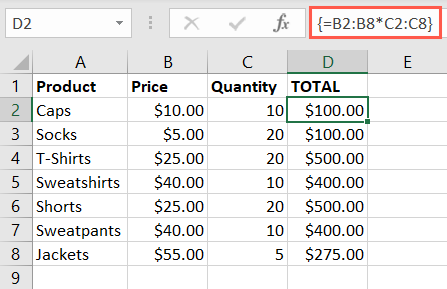
You’ll notice curly brackets surround the array formula in this case; however, the results are the same and will fill your output area.
Use the Paste Special Feature
One more way to multiply columns in Excel is with the Paste Special feature. While this method involves a few extra steps, it might just be the one you’re most comfortable using.
You’ll copy and paste one cell range into your output range. Then, copy the other cell range and use Paste Special to multiply the values.
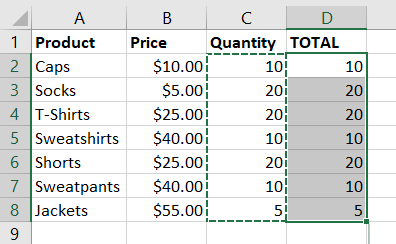
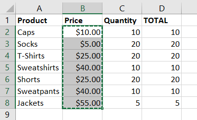
Here, we’re multiplying the values in column B (B2 through B8) by those in column C (C2 through C8) and placing the results in column D (D2 through D8). So, we’ll first copy the values in C2 through C8 and paste them in cells D2 through D8.
To do this quickly, select the cells, press Ctrl+C to copy them, go to cell D2, and press Ctrl+V to paste them.
Note: Alternatively, you can right-click and use the shortcut menu to pick the Copy and Paste actions.
Next, copy the group of cells you want to multiply by. Here, we select cells B2 through B8 and press Ctrl+C to copy them.
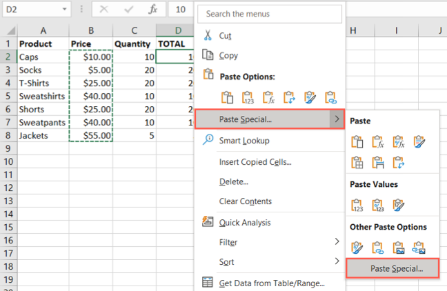
Then, go to cell D2, right-click, and pick Paste Special > Paste Special.
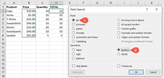
In the pop-up window, leave the default “All” marked in the Paste section and select “Multiply” in the Operation section. Click “OK.”
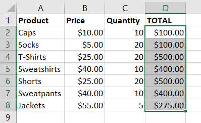
You’ll then see your columns multiplied just like using any of the other above methods.
These different methods for multiplying columns in Excel each work well. So if you’re more comfortable using the multiplication operator than the PRODUCT function or prefer the array formula over Paste Special, you’ll still get the job done.