Conditional Formatting in Excel can be considered a valuable utility that can help visually enhance the data analysis and presentation in the spreadsheet by applying particular formatting based on pre-defined rules or conditions. This post will share how you can set up conditional formatting in Excel for dates. We have also included detailed examples you can try while reading the guide.

How to set up Conditional Formatting in Excel for Dates
Conditional formatting not only helps highlight the cells using color codes but also formats the rows, columns, and cells consisting of dates in a manner that can be considered visually meaningful and appealing.
- Pre-defined
- User-defined
- Create a custom-made formatting rule
- Highlighting Holidays in Excel
- Conditional Formatting of Dates based on multiple conditions
- Highlighting upcoming Dates and Delays
Make sure to go through the details in Excel carefully. It offers many options, some of which may be beyond the scope of this guide.
1] Pre-defined conditional formatting date rules with Dates
Conditional formatting with dates can be beneficial while dealing with data sets that include date-related information. Excel provides almost ten different options to format cells based on dates, as illustrated below:
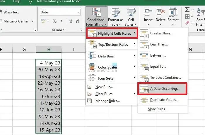
- To format a cell with the date as the Data Type, Click on Home > Conditional Formatting > Highlight Cell Rules >A Date Occurring
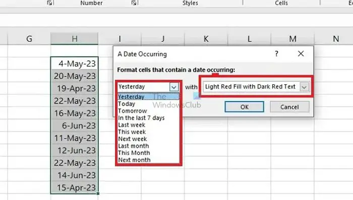
- The conditional formatting options can be chosen from the drop-down menus in the next window. The first drop-down lets us select the day range, and the formatting options can be chosen from the second one.
- Click OK to apply the formatting rules chosen.
2] User-defined conditional formatting date rules with Dates
Apart from a set of pre-defined rules, Excel also provides the option to customize these rules based on user requirements. There are multiple ways to set the customizations, as illustrated below:
Using Custom Format
- Open the A Date Occuring format window by following the steps mentioned above.
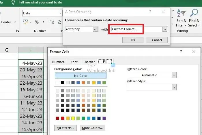
- After selecting the day range, select Custom Format from the formatting options drop-down menu.
- The Format Cells window would pop up because of the above, where we can choose the Colour, Border, Font, and Effects of our choice and then click OK to apply the changes.
Create New Rules
This method involves creating an entirely new rule for conditional formatting, unlike the above method, wherein we can choose from a few pre-defined rules and create a custom format only. Creating a new rule involves:
- Selecting the cells for which the formatting is to be applied.
- On the Home Tab, click Conditional Formatting > New Rule, which should open up the New Formatting Rule window.
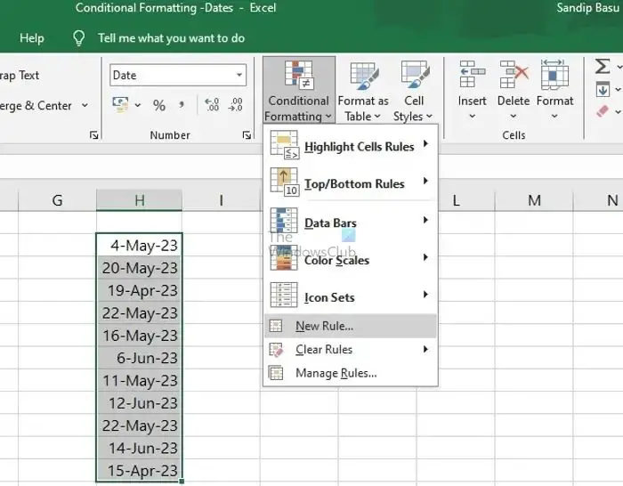
- On the said window, we can choose from the available Rule Types, followed by editing the rule description to set up the criteria for conditional formatting.
- Once completed, the Format button can be clicked on the window’s bottom-right corner to choose the formatting for the said rule.
- On the Format Cells window that opens up, we can choose the Font, Border, Cell Colour, Effects, etc., as per choice and click OK once on this window, followed by the New Formatting Rule Window for the changes to apply.
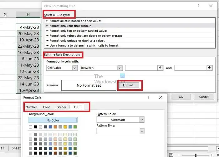
Note: The formatting rules can be used for creating and applying more than one rule for the same data set based on different conditions/criteria.
Read: Excel Date Filter is not grouping by month
3] How to create a custom-made formatting rule with dates
In the above example, we navigated the steps for creating a New Rule for Conditional Formatting based on already provided criteria. Excel also allows applying the said formatting rules on user-defined criteria.
For example, suppose we need to highlight the cells with dates that are older than 30 days or 60 days. In that case, the same can also be implemented by applying date formulas and functions available in Excel, as illustrated below:
A] Highlight Current and Older Dates
Under Select a New Rule in the Conditional Formatting option, choose Use a Formula to determine which cell to format, type:
=$H4=TODAY() to highlight the present day
=$H4>TODAY() to highlight future days
=$H4<TODAY() to highlight the previous days
=$H4<=(TODAY()-30) to highlight dates that are more than 30 days old.
=$H4<=(TODAY()-60) to highlight dates that are more than 60 days old.
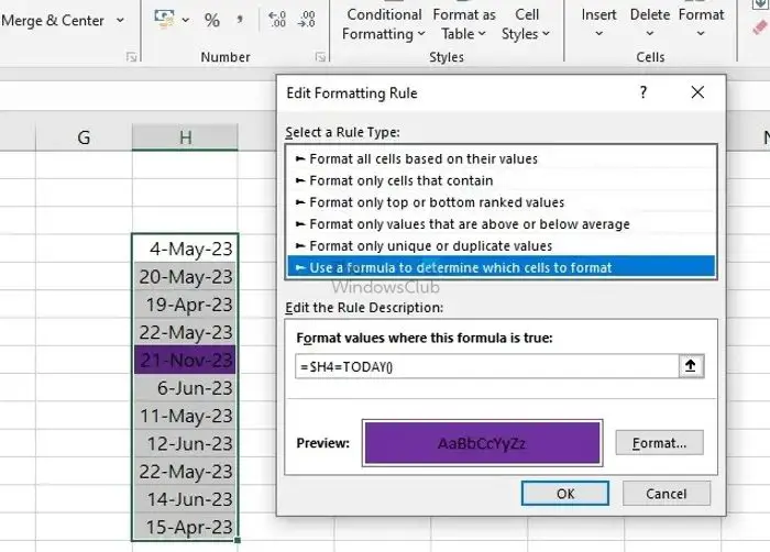
The above formula checks the selected date range for the current date, and once the match is found, change the background color to Purple as selected from the Format option. The $ used beside H signifies that the column would remain constant, but the rows would be variable.
- Once the Rule Description is mentioned, the Font, Colours, and Effects can be chosen by clicking the Format button.
- Click on OK on the Format Cells window, followed by the same on the New Rule window, for the changes to be effective.
B] Highlight based on a user-defined date range
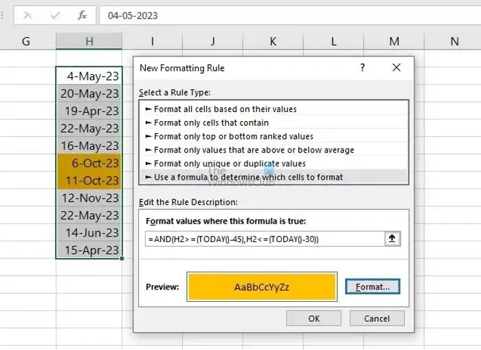
Similar methods can be applied for formatting the date ranges specified by users. For example, if we need to highlight the dates that are more than 30 days old but less than 45 days, the TODAY() function can be used in combination with a logical operator like AND to specify the criteria involving two conditions:
- Select the cells for which the formatting needs to be applied and open the New Rule window.
- In the Edit the Rule Description field, enter the below formula,
=AND(H2>=(TODAY()-45),H2<=(TODAY()-30))
The above formula uses the AND operator to highlight the dates in yellow that are more than 30 days old but less than 45 days for the entire selection, starting from cell no. H2.
C] Highlighting Weekends
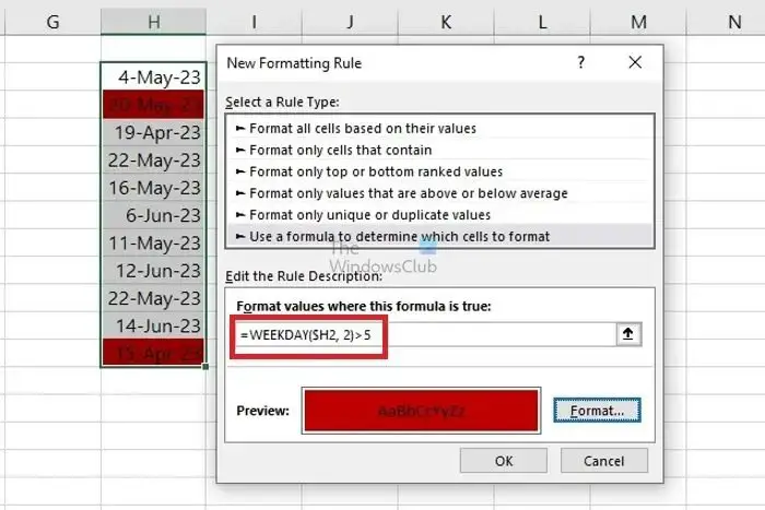
On the same range, using the WEEKDAY() formula, the dates that fall on weekends can also be highlighted:
- Select the cells for which the formatting needs to be applied and open the New Rule window.
- In the Edit the Rule Description field, enter the below formula,
=WEEKDAY($H2, 2)>5
The syntax of the Weekday formula can be represented as WEEKDAY(serial_number, [return_type]), wherein serial_number represents the cell number of the date that we are trying to check (SA1 in this case).
The return_types parameter represents the type for the week starting Monday(1) through Sunday(7), considering the start day of the week as Monday (represented by 1) and the last day of the week as Sunday ( represented by 7).
However, return_types are optional in the formula and are represented in third braces. >5 is used to highlight Saturday(6) and Sunday(7) for the specified return type.
D] Highlighting Rows Based on a Specific Date
This option can be handy while dealing with large amounts of data wherein a particular date needs to be highlighted. The same can be achieved by determining the date’s numerical value or using the DATEVALUE() function. The numerical value must be determined initially to apply conditional formatting for a specific date since Excel permanently stores dates as sequential serial numbers. To find the numerical value of a specific date,
- Right-click on the cell with the date, click on Format Cells >Number, and then choose General. A 5-digit numerical value would be displayed on the cell, which can be noted for future reference.
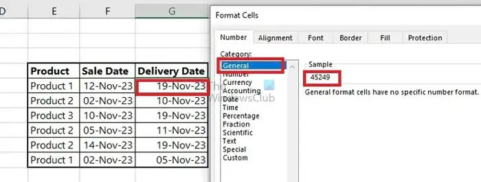
- Click on Cancel once the number is noted down since we don’t need to change the date format for the cell.
- Click on Conditional Formatting>New Rule> Select a New Rule>Use a Formula to determine which cell to format and type the following formula,
=$G5=45249
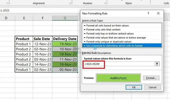
- Using the DATEVALUE() function, the same can also be done by entering the below-mentioned formula,
=$G5=DATEVALUE(“11/19/2023”)
The $ used beside C signifies that the column would remain constant, but the rows would be variable.
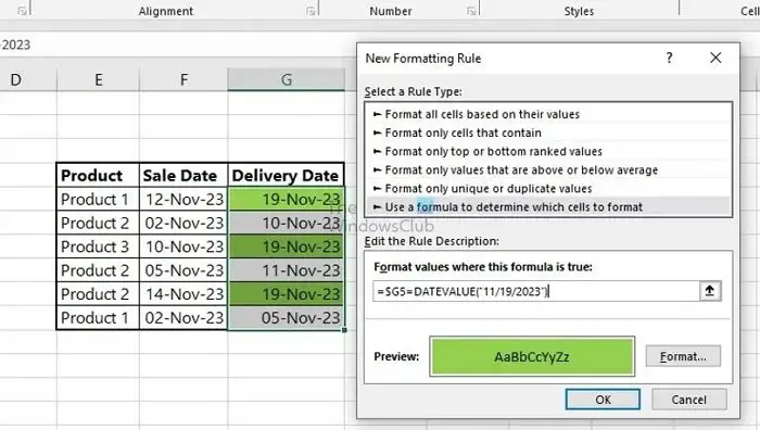
Note: The serial number sequence of these dates in Excel starts from 1st January 1900, as serial number 1. Hence, if we consider the date 19-Nov-2023, it would be numbered as 45249 since it is 45248 days after 1st January 1900.
Read: How to convert Serial Number to Date in Microsoft Excel
4] Highlighting Holidays in Excel
Since holidays may vary based on demographics, Excel doesn’t have any built-in functions to highlight public holidays. Hence, to identify the holidays, we need to have the dates recorded on a different column and apply the countif formula to check for the occurrence of the holiday dates in the datasheet.
For example, we have a few dates mentioned in column D and a list of holidays in column G. Through conditional formatting, we can highlight the holidays in RED in column D, if any, by comparing them with the holiday dates mentioned in column G using the below-mentioned steps:
- Open the New Rule dialogue box and choose Use a formula to determine which cells to format under Select Rule Type.
- Enter the formula =COUNTIF($G$3:$G$5,$D3)
- Click on Format > Fill and select the color RED from the palette and click on OK.
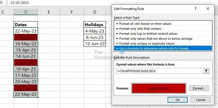
The countif() checks the occurrence of the dates mentioned in cell G3 – G5 with the dates mentioned in column D starting from cell D3.
5] Conditional Formatting of Dates based on multiple conditions
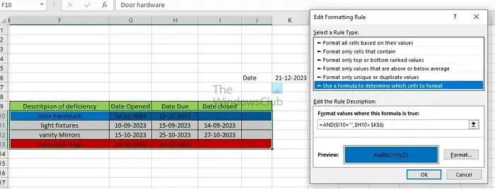
Lets assume a worksheet wherein we have complaints raised regarding various household items. The sheet features the dates when the complaints have been raised and the due and closure dates, as applicable.
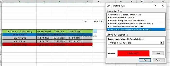
Using conditional formatting, let’s mark the complaints WHITE for the ones that have been CLOSED, RED for those that have passed the due date but not yet closed, and BLUE for those that have yet reached the due date.
The process would involve creating two conditional formatting rules for the same data, one for those that haven’t yet reached the due date and another one for those that have surpassed the due date. To do so,
- Open the conditional formatting New Rule window and select Use a formula to determine which cells to format under Select a Rule Type.
- Enter the below-mentioned formula
=AND($I10="",$H10>$K$6)
- Click Format, select the BLUE color from the palette, and click OK.
- Create another New Rule with the same rule type and enter the below-mentioned formula
=AND($I10="",$H10<$K$6)
- Click Format, select RED color from the palette, and click OK.
In this formula, we first check if the Date Closed column is BLANK or not to determine that the complaint is still open AND then check if the DUE DATE is greater than the current date or lesser to determine if the due date is approaching ($H10>$K$6) or surpassed ($H10<$K$6). The date in cell K6 represents the current date.
6] Highlighting upcoming Dates and Delays
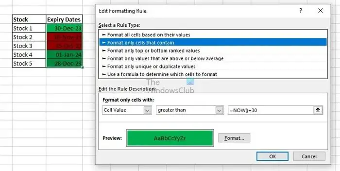
To understand how we can highlight delays with respect to dates in an Excel sheet, let us consider an example wherein we have a list of stocks with their names and expiration dates. Through conditional formatting, if we need to mark the ones that are due to expire in GREEN and the ones that have already expired in RED,
- Select the data range and open the New Rule dialogue box.
- Choose Format only cells that contain under Select Rule Type
- In Edit Rule Description, choose Cell value, Greater than, =Now()+30 in the respective dropdowns.
- Click on Format, select GREEN from the color palette, and click OK.
- Again, open a New Rule and choose the same Rule Type, as above.
- In Edit Rule Description, choose Cell value, Less than, =Now() in the respective dropdowns.
- Click on Format and select RED from the color pallet, and click OK.

Conclusion
This tutorial aims to comprehensively cover the options and functions that can be used for applying Conditional Formatting in Excel worksheets based on dates. It can help understand how to apply formatting rules to enhance data visualization and analysis. Mastering conditional formatting can also help identify trends, check deadlines, and set task priorities, helping make informed decisions.
Read: How to highlight Rows with Dates using Conditional Formatting in Excel
How do I create conditional formatting in Excel based on dates?
First, select your date cells to create conditional formatting in Excel based on dates. Click ‘Home’ > ‘Conditional Formatting’ > ‘New Rule’. Choose ‘Format cells that contain,’ select ‘Dates Occurring’ under the Rule, choose the specific date criteria, and then set your preferred format by clicking ‘Format’. Apply by hitting ‘OK’. This quickly highlights key dates in your data.
How do I conditional format due dates in Excel?
First, select your cells with dates to conditional format due dates in Excel. Then, click ‘Conditional Formatting’ from the ‘Home’ tab. Choose ‘New Rule,’ select ‘Format only cells that contain,’ set the rule to ‘Cell Value’ and ‘less than’ and enter your due date or a formula. Click ‘Format,’ pick your formatting style, and press ‘OK’ to apply.
