
If you use Google Sheets regularly, you’re probably familiar with those tools you use often. However, there are many features of this spreadsheet application that go unnoticed and underused.
Here, we’ll walk through several cool Google Sheets features that might just become your fast favorites. Head to Google Sheets, sign in with your Google account, and try out some of these hidden gems.

1. Extract Data From a Smart Chip
If you’ve taken advantage of the Smart Chips in Google’s apps, then you’ll be happy to know you can do even more with them. After you insert a Smart Chip, you can extract data from it and place it in your sheet, making chips even more useful.
You can currently extract data from People, File, and Calendar Event Smart Chips. This includes name and email, owner and filename, and summary and location.
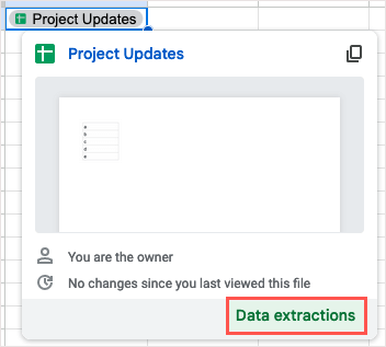
- After you insert a Smart Chip, hover your cursor over it, select it, or right-click. Then, choose Data extractions.
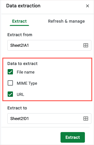
- When the sidebar opens, use the Extract tab to mark the checkboxes for those items you want to extract.
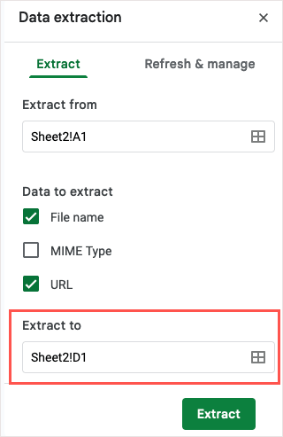
- Use the Extract to field to enter or select the sheet location where you want the data.
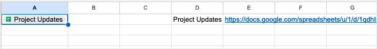
- Pick Extract and you’ll see your data display in your selected location.
If you need to refresh the extracted data, you can use the Refresh & manage tab in the sidebar.
2. Create a QR Code
QR codes are popular ways to share information, direct people to your website, and even provide discounts. By creating your own QR code in Google Sheets without add-ons or third-party tools, you or your collaborators can quickly take action.
To make the QR code, you’ll use the Google Sheets IMAGE function and a link to Google’s root URL: https://chart.googleapis.com/chart?.
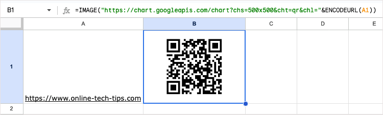
Here, we’ll link to the website in cell A1 using the formula below. Place the formula in the cell where you want the QR code.
=IMAGE(“https://chart.googleapis.com/chart?chs=500×500&cht=qr&chl=”&ENCODEURL(A1))
Use the following arguments to build your formula:
- CHS argument: Define the dimensions of the QR code in pixels (chs=500×500).
- CHT argument: Specify a QR code (cht=qr).
- CHL argument: Choose the URL data (chl=”&ENCODEURL(A1)).
Then, use the ampersand operator (&) to connect the arguments.
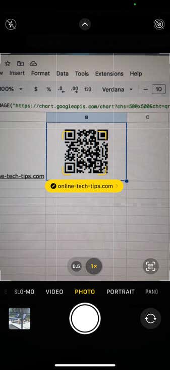
Once you see the code, you may need to resize the row and/or column to view its full size. Then, scan the QR code to make sure it works as you expect.
You can also use optional arguments for encoding the data in a particular way or assigning a correction level. For more on these arguments, check out the Google Charts Infographics reference page for QR codes.
3. Insert a Drop-Down List
Drop-down lists are terrific tools for data entry. By selecting an item from a list, you can make sure you’re entering the data you want and can reduce errors at the same time.
Since the introduction of drop-down lists in Sheets, the feature has been enhanced to give you a simpler way to create and manage these helpful lists.
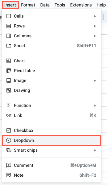
- Insert a drop-down list by doing one of the following:
- Select Insert > Dropdown from the menu.
- Right-click and choose Dropdown.
- Type the @ (At) symbol and choose Dropdowns in the Components section.
- You’ll then see the Data Validation Rules sidebar open. Enter the location for the list in the Apply to range box and confirm that Dropdown is selected in the Criteria drop-down menu.
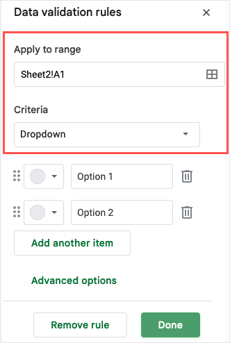
- Then, add your list items in the Option boxes and optionally select colors for them to the left.
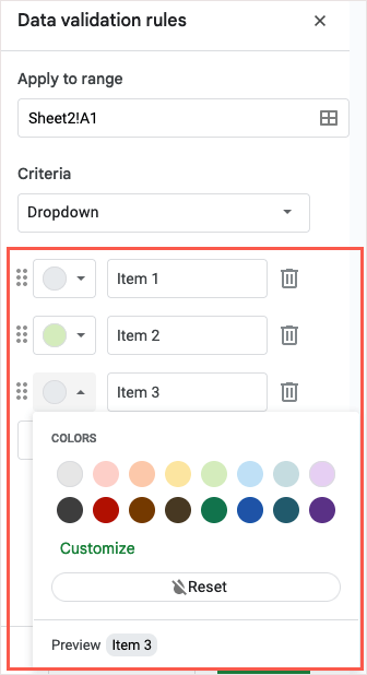
- To display help text, pick the action for invalid data, or choose the display style, expand the Advanced Options section.
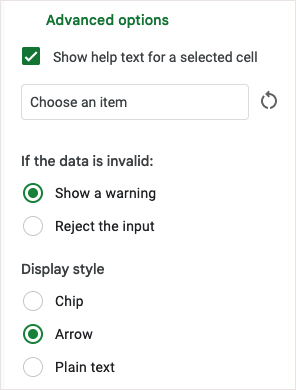
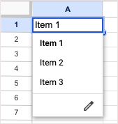
- When you finish, select Done. Then, use your new drop-down list to enter data in your sheet.
4. Validate an Email Address
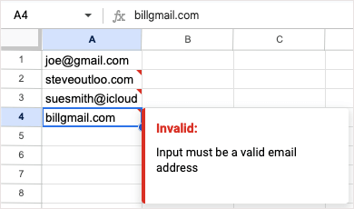
When you have a spreadsheet that contains email addresses, whether Gmail, Outlook, or something else, you may want to make sure they’re valid. While Sheets doesn’t show you if an address is legitimate, it does show you if it’s formatted correctly with the @ (At) symbol and a domain.
- Select the cell(s) you want to check and go to Data > Data validation in the menu.

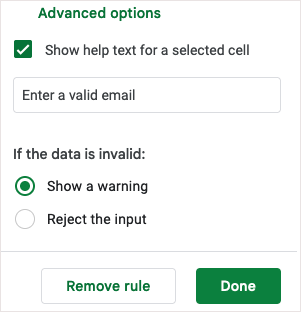
- When the Data Validation Rules sidebar opens, select Add rule, confirm or adjust the cells in the Apply to range field, and choose Text is valid email in the Criteria drop-down box.

- Optionally select the Advanced Options such as showing help text, displaying a warning, or rejecting the input. Pick Done to save and apply the validation rule.
You can then test the validation and options by entering an invalid email address.
5. Make a Custom Function
Are you a fan of using functions and formulas in Google Sheets? If so, why not create your own? Using the Custom Function feature, you can set up your own function and reuse it whenever you like.
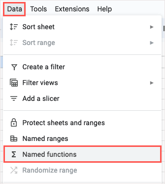
- Select Data > Named functions from the menu.
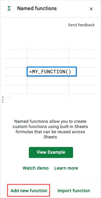
- In the Named Functions sidebar that opens, use Add new function at the bottom to create your custom function. You can also look at an example, watch the demonstration, or find out more about the feature.
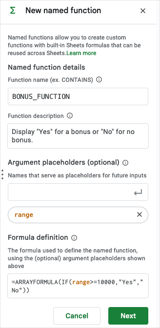
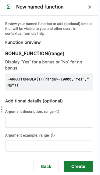
- Enter the function name, description, and optionally argument placeholders. Enter the formula you want to use to define the function and select Next.
- Check out the Function preview and either select Back to make changes or Create to save the new function. Notice you can also add optional arguments if necessary.
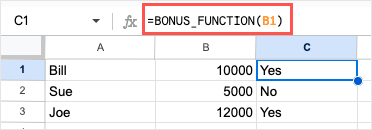
- You’ll then see the function in the sidebar list. Enter it into a cell in your sheet to test it out.
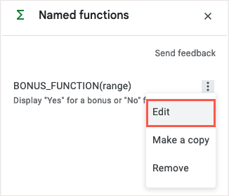
If you need to make edits, reopen the Named Functions sidebar, select the three dots to the right of the function, and pick Edit.
6. Use a Slicer to Filter a Chart
Charts give you handy and effective ways to display your data. Using a slicer, you can filter the data that displays in the chart. This is convenient for reviewing specific portions of the chart data when needed.
Insert a Slicer
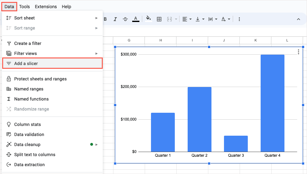
After you insert your chart, select it and go to Data > Add a slicer in the menu.
When the sidebar opens, open the Data tab, confirm the Data Range at the top, and then pick the Column to use for the filter.
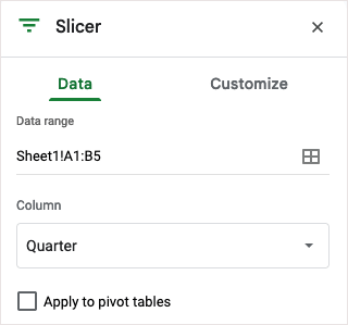
You’ll see the slicer appear as a black rounded rectangle which you can move or resize as you please.
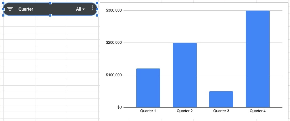
Use a Slicer
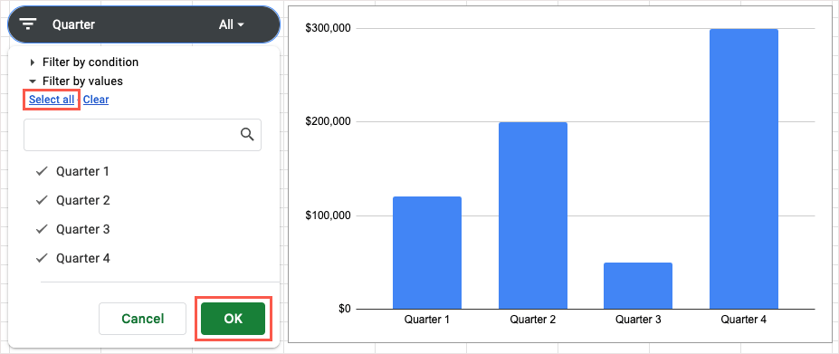
Once you have your slicer, select the Filter button on the left or drop-down arrow on the right. Then, select the data you want to see in the chart which places checkmarks next to those items.
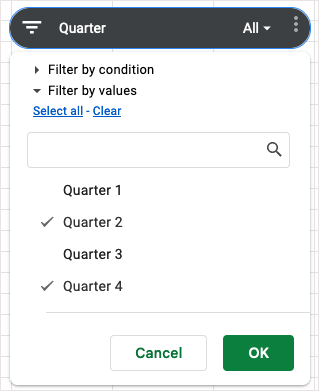
Select OK and you’ll see your chart update immediately.
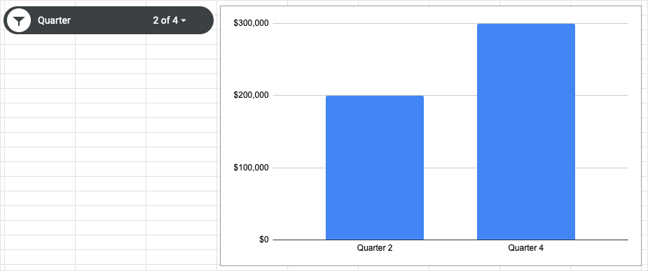
To return your chart to the original view showing all data, open the filter and pick Select all > OK.
7. Quickly Calculate Data
Sometimes you want to see a quick calculation without adding a formula to your sheet. In Google Sheets, you can simply select the values and then choose a calculation to view without any extra work.
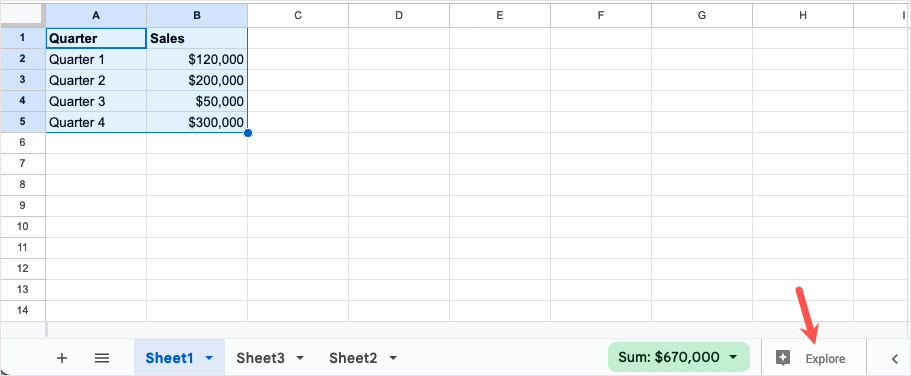
- Select the data you want to calculate and then look on the bottom right of the tab row. You’ll see the calculation menu in green which contains the Sum of your data.
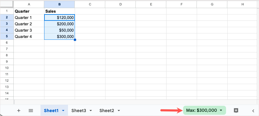
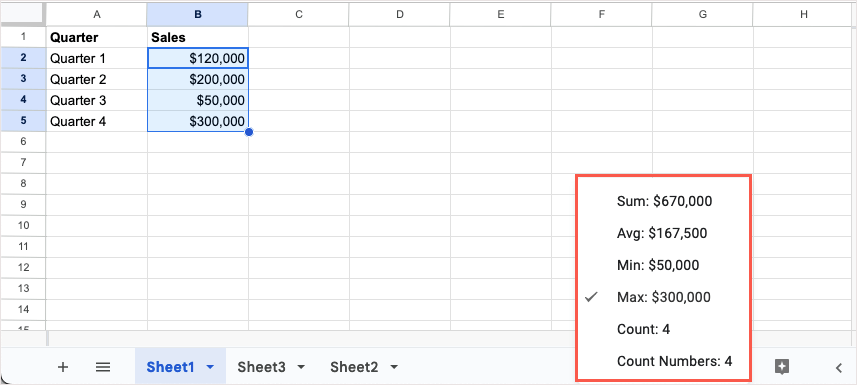
- Open that menu and choose the calculation you want to perform. You’ll see the new result in that menu.

- You can also simply open the menu to see all available calculations in real-time.
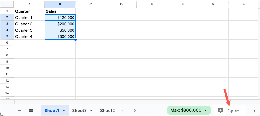
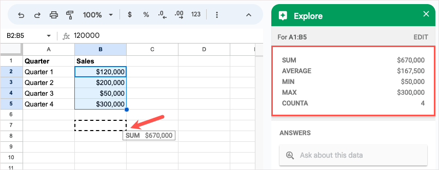
If you decide to include the calculation in your sheet, keep the cell selected and choose Explore to the right of the sheet tabs.
When the sidebar opens, drag the calculation you want to use to a cell in your sheet.
8. Explore Ways to Present Your Data
Maybe you have data in your spreadsheet but aren’t sure of the best way to display or analyze it. With the Explore feature, you can see various quick ways to present your data, review details about it, and ask questions.
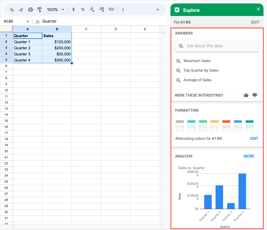
Select your data and pick Explore on the bottom right.
When the Explore sidebar opens, you’ll see options for your data. Type a question in the Answers section, apply color using the Formatting section, or insert a chart from the Analysis section.
After you finish, simply use the X on the top right of the sidebar to close it.
9. Request Sheet Approvals
If you use a Google Workspace account for business or education, check out the Approvals feature. With it, you can request approvals from others and keep track of what’s approved and what isn’t.
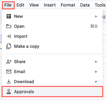
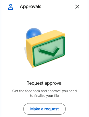
Go to File and select Approvals.
When the Approvals sidebar opens, choose Make a request.
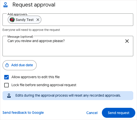
In the pop-up window, add those you want to approve your request and optionally a message. You can also include a due date, allow the approvers to edit the sheet, or lock the file before sending your request for approval. Choose Send request when you finish.
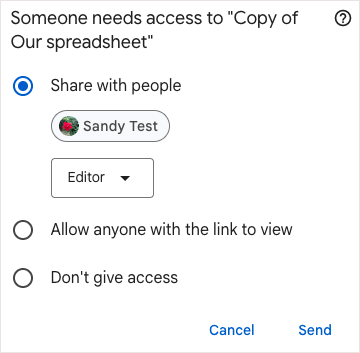
If you haven’t shared the document with the approvers already, you’ll be asked to do so and assign the permissions.
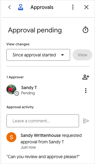
You can then view the status by returning to the Approvals sidebar.
10. Set Up a Custom Date and Time Format
While Google Sheets provides many different ways to format your dates and times, maybe you want something in particular. You can create your own date and time format with the structure, colors, and style you want.
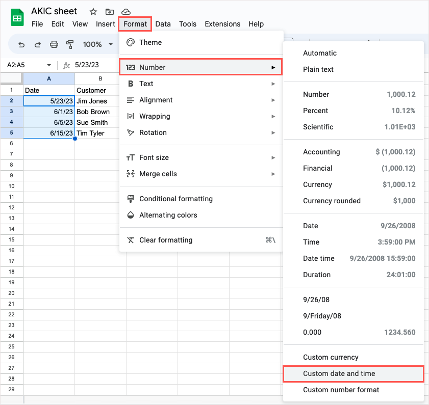
- Select the cell(s) containing the date or time and go to Format > Number > Custom date and time. Alternatively, you can select the More Formats option in the toolbar and pick Custom date and time.
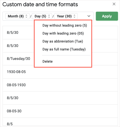
- When the window opens, you’ll see the current format for your date and/or time. Select an existing element at the top to change the format or delete it.
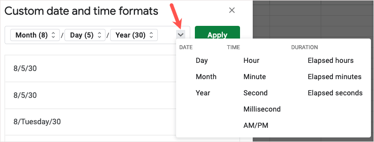
- To add a different element, select the arrow on the right side and choose one from the list. You can then format that element using its arrow.
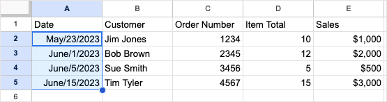
- When you finish, select Apply to use the custom date and time format and you should see your sheet update.
With these Google Sheets features, you can do even more with your data. Be sure to try one or more and see which come in handy for you.
For related tutorials, look at how to find duplicates in Google Sheets using the conditional formatting options.